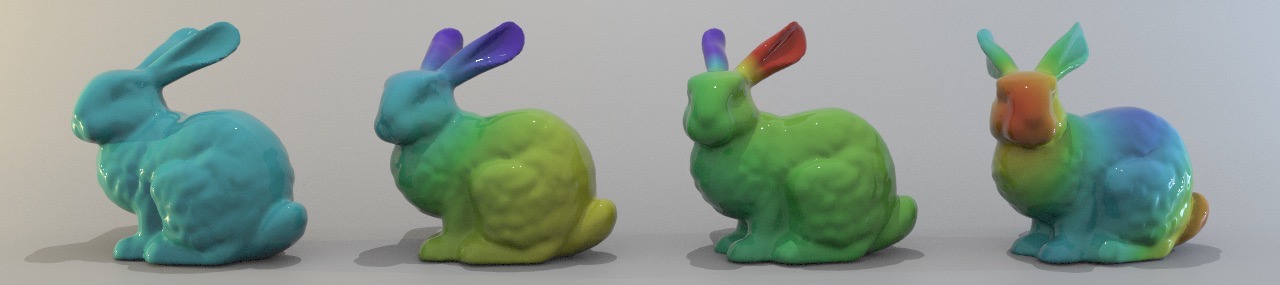
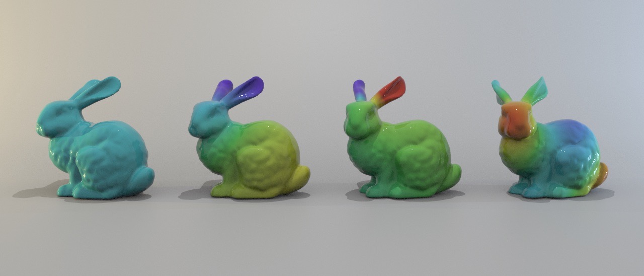
Below is an image of four of the harmonic modes of the Stanford
bunny. From left to right, I've plotted the \(0^{th}\), \(1^{st}\), \(2^{nd}\), and \(6^{th}\) modes. I computed the
displacement \(u\) of each mode by numerically solving the Helmholtz equation, \( \Delta u = -k^2 u \), at every vertex on
the triangulated surface. The purple portions represent regions where the displacement is maximally negative, and the red portions
represent where it is maximally positive. In discrete exterior calculus,
the Helmholtz equation takes the form
$$(d^T \star_1 d) u = k^2 \star_0 u $$
where \(d^T \star_1 d\) is the discrete Laplacian, \(\star_0\) is the mass matrix, and \(k\) is the wave number of the harmonic mode. Here,
\(d\) is a sparse matrix defined using the source and destination of each half edge on the mesh, \(\star_1\)
is a sparse diagonal matrix whose non-zero values are the half edge weights, and \(\star_0\) is a sparse diagonal matrix
whose non-zero values are the vertex weights. The computation was performed using VEX and Python, and the
graphics were rendered using Houdini. Note: if the bunnies were replaced by spheres, the
eigenvectors \(u\) would be the corresponding real spherical harmonics.
Musical Instruments
Strings, membranes, and plates are the basic building
blocks of musical instruments. Using modal synthesis and finite-difference time-domain (FDTD) methods, I simulated sounds
corresponding to each of these musical instrument objects. In the case of plates, I modeled different materials and
excitation mechanisms. Audio samples of each musical instrument object are provided below. For future work, I plan to
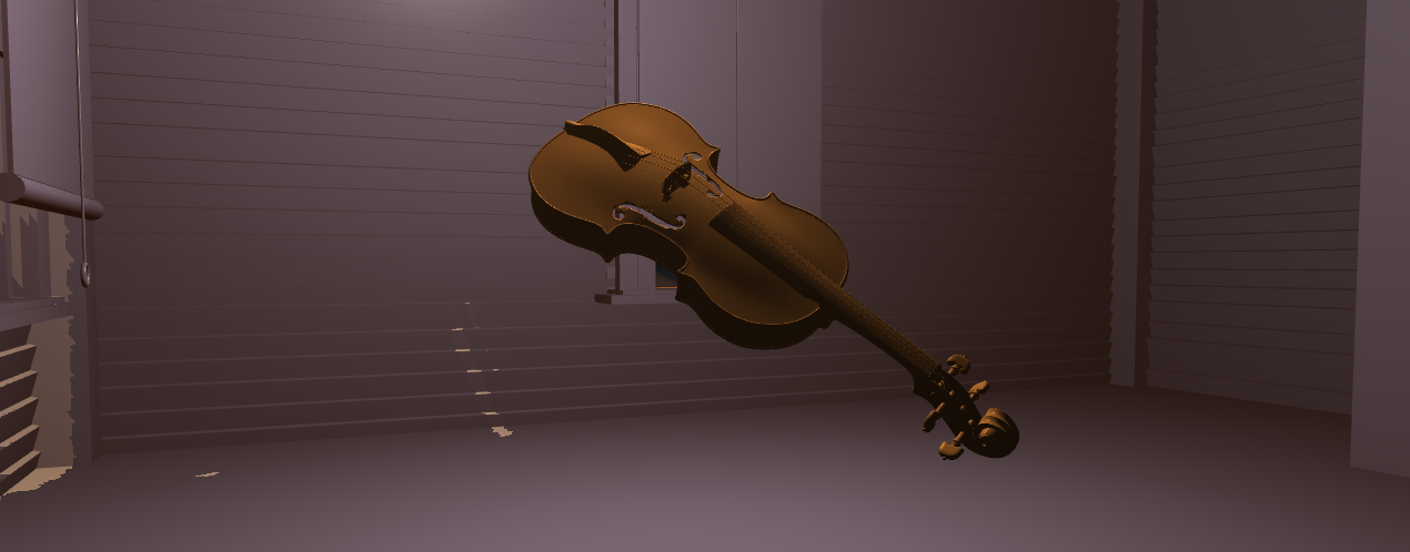
integrate the sounds into virtual reality. In preparation, I have graphically rendered musical instruments to use as
interaction models (see violin below).
String
Membrane
Plate
Speech
Wolfgang von Kempelen created the first known speech synthesizer in 1791. The device used a variety of parts to
imitate human speech—a bellows for the lungs, a reed for the vocal folds, tubes for the various vocal-tract geometries,
and so on. By reproducing the subtleties of linguistic sounds from observations of the acoustic and physiological
mechanisms of speech, Kempelen set the stage for more advanced speech synthesis techniques that would emerge
centuries later.
Physical modeling speech synthesis is a computational approach to artificial voice production that generates
acoustic sounds by numerically solving a mathematical model of speech. As part of my special project
dissertation in Acoustics and Music Technology at the University of Edinburgh,
I developed physical modeling simulations of vocal-tract sound propagation by solving Webster's equation with
finite-difference time-domain (FDTD) methods. For another course project, I also created a unit selection speech
synthesizer, which concatenates individual diphones of speech. Code from my
FDTD and unit selection
speech synthesizers is available on my GitHub page. To demonstrate my simulations, I used the English phrase I owe you a yo-yo.
I chose this phrase because it contains only vowels and diphthongs. Other speech sounds, like consonants
and glottal fry, were left for future research. Similar to musical instrument synthesis discussed above, I plan to synchronize
speech sounds with facial animations.
FDTD Speech
Unit Selection
References
C. McKell. Finite-Difference Simulations of Speech with Wall Vibration Losses , Special Project Master's Dissertation, University of Edinburgh, Acoustics and Audio Group, April 2017. [paper]
Sound Synthesis for Computer Animation
The images, motion, and sounds of the animation below
were generated entirely by a computer. The images were computed at 60 Hz, the motion was computed at 240 Hz, and the
sounds were computed at 48,000 Hz. Each sound event consisted of a pure tone modified by an attack-decay-release (ASR)
volume envelope. From left to right in the animation, the spheres played frequencies of 220 Hz, 440 Hz, and 880 Hz. Following the main computation,
the audio and video were automatically combined using FFmpeg. The computation was performed using C++, and the
graphics were rendered using OpenGL. The main computation took the following general form:
for (int i = 0; i < 60; i++) {
// render images of falling spheres at 60 Hz
for (int k = 0; k < numberOfSpheres; k++) {
// advance position of each sphere using forward Euler method
// initialize new sound event if sphere collides with floor
for (int w = 0; w < 200; w++) {
// compute audio samples for each sound event at 60 \(\times\) 4 \(\times\) 200 = 48,000 Hz
}
}
}
}